ADM-EC Clock Consensus
Delay-Constrained Anomaly-Aware Consensus in Heterogeneous Clock Networks
View the Project on GitHub threehouse-plus-ec/admec-clock-consensus
WP1 Tutorial: Information Content for Clock Data
Time to run: ~2 minutes on a laptop.
Audience: Graduate student or postdoc in physics who knows Python and basic statistics but has never heard of IC.
What this covers: The core WP1 arc — defining IC, calibrating it under null conditions, understanding its limitations, and positioning it against familiar figures of merit.
What this does not cover: The full calibration runs (300 realisations x 10 models). For those, see the logbook entries and the data archive.
The problem
Modern timekeeping relies on networks of clocks that continuously compare their readings and agree on a shared timescale. The best optical clocks now reach fractional uncertainties below 10^{-18} — sensitive enough to detect height differences of a few centimetres through gravitational time dilation.
At this precision, clocks disagree. The standard response is robust averaging: suppress outliers so the consensus remains stable. This works when deviations are random noise.
But what if some disagreements carry information? A clock drifting systematically might indicate an environmental change. By suppressing it, we lose that signal. This project asks whether distinguishing structured anomalies (persistent drifts, growing variance) from unstructured ones (random outliers) — and treating them differently — improves consensus. The first step is to define and calibrate a measure of how surprising each reading is. That measure is information content (IC).
For the non-technical version, see the outreach document. For the full technical record, see the WP1 summary.
1. Setup
The codebase is small: three implemented modules in src/. We’ll use all three.
import sys, os
sys.path.insert(0, os.path.join(os.getcwd(), '..', 'src'))

import numpy as np
import matplotlib.pyplot as plt
from scipy.stats import norm as norm_dist

from ic import compute_ic, compute_aipp, aipp_gaussian_limit, perturb_sigmas
from noise import generate_pareto_symmetric, generate_flicker, generate_random_walk, generate_ar1
from temporal import compute_temporal_structure, calibrate_delta_min

# Reproducibility
rng = np.random.default_rng(2026)

# Plotting defaults
plt.rcParams.update({'figure.dpi': 100, 'font.size': 11})

print(f"Modules loaded. NumPy {np.__version__}.")
Modules loaded. NumPy 1.23.5.
2. What is IC?
A single clock produces N readings over time, each with a declared measurement uncertainty. IC asks: how consistent is each reading with the clock’s own track record?
The idea is simple. We build a background density from all N readings — a Gaussian mixture where each reading contributes one component — and then ask how much probability mass that density assigns to the neighbourhood of each individual reading. Readings that sit in low-density regions of the mixture get high IC.
Formally, for N readings $x_1, \ldots, x_N$ with uncertainties $\sigma_1, \ldots, \sigma_N$:
\[P(y) = \frac{1}{N} \sum_{i=1}^{N} \mathcal{N}(y;\, x_i,\, \sigma_i)\]The interval probability for reading $k$ is:
\[p_k = \int_{x_k - \sigma_k}^{x_k + \sigma_k} P(y)\, dy\]And the information content is:
\[I_k = -\log_2(p_k) \quad [\text{bits}]\]Let’s see this in action. We’ll generate 50 Gaussian readings, build P(y), and show how a tail reading gets high IC.
# Generate 50 Gaussian readings with sigma = 1
N = 50
values = rng.normal(0, 1, N)
sigmas = np.ones(N)

# Build P(y) explicitly for plotting
y_grid = np.linspace(-4, 4, 500)
P_y = np.zeros_like(y_grid)
for i in range(N):
    P_y += norm_dist.pdf(y_grid, values[i], sigmas[i])
P_y /= N

# Pick one point to illustrate: the one furthest from zero
k = np.argmax(np.abs(values))
x_k, sigma_k = values[k], sigmas[k]

# Compute IC for all points
ic = compute_ic(values, sigmas)

# --- Figure: P(y) with the interval for point k highlighted ---
fig, (ax1, ax2) = plt.subplots(1, 2, figsize=(13, 4.5))

# Left: the mixture density and the interval
ax1.plot(y_grid, P_y, 'k-', linewidth=1.5, label='$P(y)$ (Gaussian mixture)')
ax1.fill_between(y_grid, P_y,
                 where=(y_grid >= x_k - sigma_k) & (y_grid <= x_k + sigma_k),
                 alpha=0.4, color='tomato',
                 label=f'Interval for reading k={k}\n'
                       f'$x_k$ = {x_k:.2f}, $p_k$ = {2**(-ic[k]):.4f}')
ax1.axvline(x_k, color='tomato', linestyle=':', linewidth=1)
ax1.set_xlabel('y')
ax1.set_ylabel('P(y)')
ax1.set_title('Gaussian-mixture background density')
ax1.legend(fontsize=9)

# Right: IC vs value
ax2.scatter(values, ic, c='teal', s=25, alpha=0.7)
ax2.scatter(values[k], ic[k], c='tomato', s=80, zorder=5,
            label=f'Reading k={k}: IC = {ic[k]:.2f} bits')
ax2.set_xlabel('Value $x_k$')
ax2.set_ylabel('IC (bits)')
ax2.set_title('IC per reading')
ax2.legend(fontsize=9)

plt.tight_layout()
plt.show()

print(f"Reading k={k}: value = {x_k:.2f}, IC = {ic[k]:.2f} bits")
print(f"Points near zero have low IC; points in the tails have high IC.")
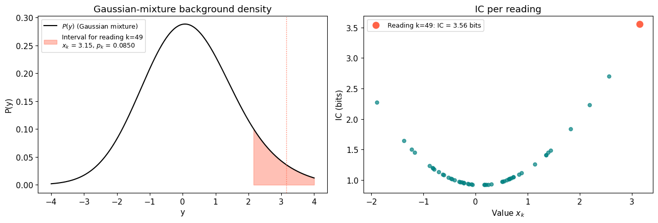
Reading k=49: value = 3.15, IC = 3.56 bits
Points near zero have low IC; points in the tails have high IC.
3. The outlier demo
A practical sanity check: if we inject two obvious outliers into otherwise well-behaved data, IC should flag them. This is fig03 from logbook Entry 001, rebuilt live.
# 40 Gaussian points with two injected outliers
n = 40
values_demo = rng.normal(0, 1, n)
values_demo[35] = 6.0
values_demo[37] = -5.5
sigmas_demo = np.ones(n)

ic_demo = compute_ic(values_demo, sigmas_demo)
threshold_95 = np.percentile(ic_demo, 95)

fig, (ax1, ax2) = plt.subplots(2, 1, figsize=(10, 5.5), sharex=True)

# Data
markerline, stemlines, baseline = ax1.stem(range(n), values_demo, linefmt='b-',
                                            markerfmt='bo', basefmt='gray')
plt.setp(stemlines, linewidth=1)
plt.setp(markerline, markersize=4)
for idx in [35, 37]:
    ax1.annotate('outlier', xy=(idx, values_demo[idx]),
                 xytext=(idx + 0.5, values_demo[idx] + (0.5 if values_demo[idx] > 0 else -0.5)),
                 fontsize=9, color='red', fontweight='bold',
                 arrowprops=dict(arrowstyle='->', color='red', lw=1))
ax1.set_ylabel('Value')
ax1.set_title('(a) Data with two injected outliers')
ax1.axhline(0, color='gray', linewidth=0.5)

# IC
markerline, stemlines, baseline = ax2.stem(range(n), ic_demo, linefmt='-',
                                            markerfmt='o', basefmt='gray')
plt.setp(stemlines, color='darkorange', linewidth=1)
plt.setp(markerline, color='darkorange', markersize=4)
ax2.axhline(threshold_95, color='gray', linestyle='--', linewidth=1, label='95th percentile')
ax2.set_xlabel('Reading index')
ax2.set_ylabel('IC (bits)')
ax2.set_title('(b) Information Content per reading')
ax2.legend(fontsize=9)

plt.tight_layout()
plt.show()

print(f"Outlier at index 35 (value=6.0):  IC = {ic_demo[35]:.2f} bits")
print(f"Outlier at index 37 (value=-5.5): IC = {ic_demo[37]:.2f} bits")
print(f"Median IC of normal points:       {np.median(ic_demo[np.array([i for i in range(n) if i not in [35,37]])]):.2f} bits")
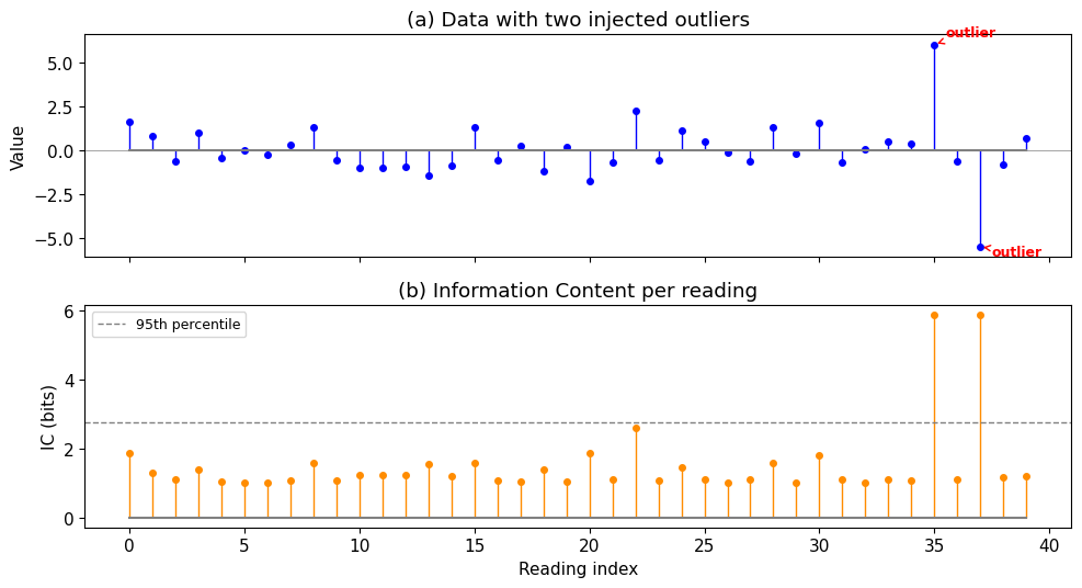
Outlier at index 35 (value=6.0):  IC = 5.86 bits
Outlier at index 37 (value=-5.5): IC = 5.86 bits
Median IC of normal points:       1.11 bits
4. How does AIPP behave under the null?
AIPP (average information per point) is the ensemble-level summary: the mean IC across all N readings. Under the Gaussian null, AIPP converges to a theoretical limit as N grows.
The key insight: as N increases, the Gaussian mixture P(y) converges to a broader distribution than any single component — specifically, to $\mathcal{N}(0, \sqrt{2})$ when $\sigma_\text{data} = \sigma_\text{declared} = 1$. This is the convolution of the data distribution with the Gaussian kernel. The broader background means each reading’s interval captures less probability mass, giving higher IC.
An earlier version of the project proposal incorrectly claimed AIPP $\to$ 0.55 bit, based on considering only the self-contribution of each reading. The correct value is 1.25 bit. See logbook Entry 001 for the full derivation.
# AIPP convergence: compute at increasing N (50 realisations each, for speed)
Ns = [5, 10, 20, 50, 100, 200, 500, 1000]
n_real = 50
rng_conv = np.random.default_rng(2026)

means, stds = [], []
for n in Ns:
    aipps = [compute_aipp(compute_ic(rng_conv.normal(0, 1, n), np.ones(n)))
             for _ in range(n_real)]
    means.append(np.mean(aipps))
    stds.append(np.std(aipps))

means, stds = np.array(means), np.array(stds)
limit = aipp_gaussian_limit()  # theoretical ~1.25 bit

from scipy.special import erf
old_claim = -np.log2(erf(1.0 / np.sqrt(2.0)))  # the incorrect 0.55 bit

fig, ax = plt.subplots(figsize=(8, 4.5))
ax.errorbar(Ns, means, yerr=stds, fmt='o-', color='teal', markersize=5,
            capsize=3, label=f'Empirical ({n_real} realisations)')
ax.axhline(limit, color='darkorange', linewidth=1.5,
           label=f'Correct limit = {limit:.2f} bit')
ax.axhline(old_claim, color='gray', linewidth=1, linestyle='--',
           label=f'Old (wrong) claim = {old_claim:.2f} bit')
ax.axhspan(limit * 0.95, limit * 1.05, color='darkorange', alpha=0.12,
           label='$\pm$5% band (DG-1 criterion)')
ax.set_xlabel('N (number of readings)')
ax.set_ylabel('AIPP (bits)')
ax.set_title('AIPP convergence under Gaussian null')
ax.legend(fontsize=9)
ax.set_ylim(0, 2.0)
plt.tight_layout()
plt.show()

print(f"Theoretical limit: {limit:.4f} bit")
print(f"At N=100: AIPP = {means[Ns.index(100)]:.3f} +/- {stds[Ns.index(100)]:.3f}")
print(f"At N=1000: AIPP = {means[Ns.index(1000)]:.3f} +/- {stds[Ns.index(1000)]:.3f}")
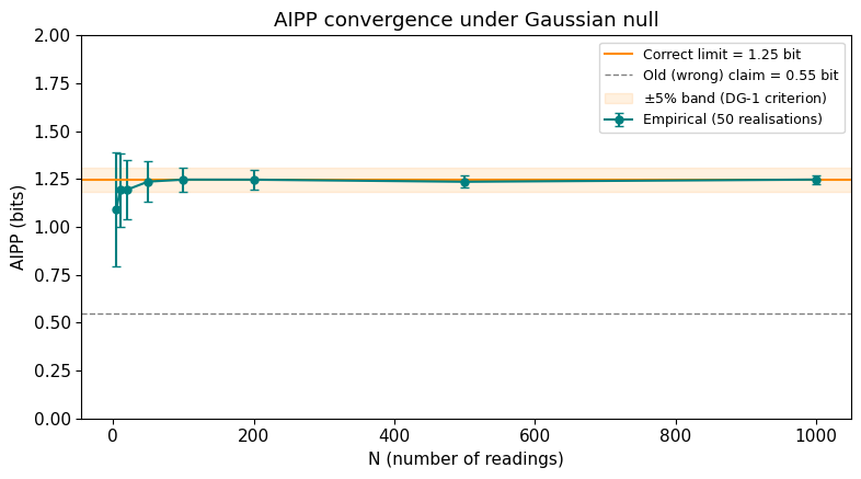
Theoretical limit: 1.2482 bit
At N=100: AIPP = 1.247 +/- 0.064
At N=1000: AIPP = 1.247 +/- 0.023
5. Is IC robust across noise types?
A useful anomaly detector shouldn’t require knowing the exact noise model. We test IC under four contrasting distributions: Gaussian (the baseline), Student-t with 3 degrees of freedom (heavy tails), AR(1) with $\rho = 0.9$ (strong temporal correlation), and random walk (non-stationary).
The DG-1 criterion requires that 95th-percentile thresholds remain within a factor of 1.5 across noise models. The full calibration (10 models, 300 realisations each) is in logbook Entry 003. Here we run a quick version with 4 models and 50 realisations.
N_thr = 50
n_real_thr = 50
rng_thr = np.random.default_rng(2026)

models = {
    'Gaussian': lambda: (rng_thr.normal(0, 1, N_thr), np.ones(N_thr)),
    'Student-t(3)': lambda: (rng_thr.standard_t(3, N_thr), np.ones(N_thr) * np.sqrt(3)),
    'AR(1) p=0.9': lambda: (generate_ar1(N_thr, rho=0.9, rng=rng_thr), np.ones(N_thr)),
    'Random walk': lambda: (generate_random_walk(N_thr, rng=rng_thr),
                            np.maximum(np.sqrt(np.arange(1, N_thr + 1, dtype=float)), 1.0)),
}

results = {}
for name, gen in models.items():
    aipps = []
    for _ in range(n_real_thr):
        v, s = gen()
        aipps.append(compute_aipp(compute_ic(v, s)))
    results[name] = np.array(aipps)

# Plot
fig, ax = plt.subplots(figsize=(8, 4.5))
labels = list(results.keys())
data = [results[l] for l in labels]
colors = ['#5DA5DA', '#F15854', '#60BD68', '#FAA43A']
bp = ax.boxplot(data, labels=labels, patch_artist=True, widths=0.5,
                medianprops=dict(color='black', linewidth=1.5))
for patch, c in zip(bp['boxes'], colors):
    patch.set_facecolor(c)
    patch.set_alpha(0.7)

# Mark 95th percentiles
p95s = [np.percentile(d, 95) for d in data]
ax.scatter(range(1, len(p95s) + 1), p95s, marker='v', color='darkred',
           s=60, zorder=5, label='95th percentile')

gaussian_p95 = p95s[0]
ax.axhspan(gaussian_p95 / 1.5, gaussian_p95 * 1.5, color='gray', alpha=0.1,
           label=f'x1.5 band (DG-1)')
ax.axhline(gaussian_p95, color='gray', linestyle='--', linewidth=0.8)

ax.set_ylabel('AIPP (bits)')
ax.set_title(f'Threshold stability across noise models (N={N_thr}, {n_real_thr} realisations)')
ax.legend(fontsize=9)
plt.tight_layout()
plt.show()

# Print the ratio
max_p95 = max(p95s)
min_p95 = min(p95s)
print(f"95th-percentile range: {min_p95:.3f} to {max_p95:.3f}")
print(f"Max pairwise ratio: {max_p95/min_p95:.2f}x (DG-1 requires < 1.5x)")
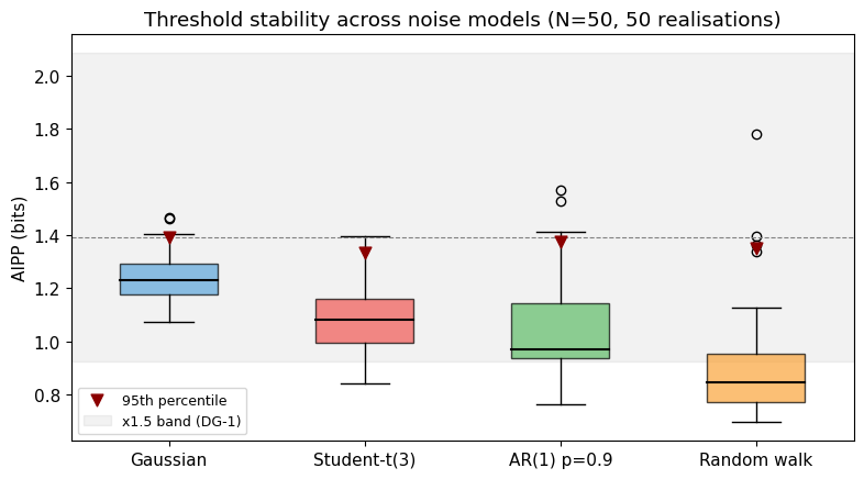
95th-percentile range: 1.333 to 1.390
Max pairwise ratio: 1.04x (DG-1 requires < 1.5x)
6. What happens when $\sigma$ is wrong?
IC depends on the declared uncertainty $\sigma_k$ — it sets both the width of each mixture component and the integration interval. What happens when $\sigma$ is systematically wrong?
We test three perturbation conditions against the unperturbed baseline:
- Random $\pm$20%: each $\sigma_k$ is independently perturbed by a random factor in $[-0.2, +0.2]$.
- Systematic +20%: all $\sigma_k$ are overestimated by 20%.
- Systematic $-$20%: all $\sigma_k$ are underestimated by 20%.
The pre-registered bound is 15% AIPP shift. See logbook Entry 002 for the full analysis.
N_sens = 200
n_real_sens = 100
rng_sens = np.random.default_rng(2026)

conditions = [
    ('Unperturbed', None),
    ('Random +/-20%', 'random'),
    ('Systematic +20%', 'systematic+'),
    ('Systematic -20%', 'systematic-'),
]

sens_results = {}
for label, mode in conditions:
    aipps = []
    for _ in range(n_real_sens):
        v = rng_sens.normal(0, 1, N_sens)
        s_true = np.ones(N_sens)
        s_used = s_true if mode is None else perturb_sigmas(s_true, mode=mode,
                                                             magnitude=0.2, rng=rng_sens)
        aipps.append(compute_aipp(compute_ic(v, s_used)))
    sens_results[label] = np.array(aipps)

# Plot
fig, ax = plt.subplots(figsize=(8, 4.5))
labels = list(sens_results.keys())
data = [sens_results[l] for l in labels]
colors = ['#5DA5DA', '#FAA43A', '#60BD68', '#F15854']
bp = ax.boxplot(data, labels=labels, patch_artist=True, widths=0.5,
                medianprops=dict(color='black', linewidth=1.5))
for patch, c in zip(bp['boxes'], colors):
    patch.set_facecolor(c)
    patch.set_alpha(0.7)

baseline = np.mean(sens_results['Unperturbed'])
ax.axhspan(baseline * 0.85, baseline * 1.15, color='gray', alpha=0.12,
           label='$\pm$15% of baseline')
ax.axhline(baseline, color='gray', linestyle='--', linewidth=0.8)

ax.set_ylabel('AIPP (bits)')
ax.set_title(f'$\\sigma$-sensitivity (N={N_sens}, {n_real_sens} realisations)')
ax.legend(fontsize=9)
plt.tight_layout()
plt.show()

# Print shifts
print(f"{'Condition':<22} {'Mean AIPP':>10} {'Shift':>8}")
print("-" * 44)
for label in labels:
    m = np.mean(sens_results[label])
    shift = (m - baseline) / baseline * 100
    flag = " <-- FAIL" if abs(shift) > 15 else ""
    print(f"{label:<22} {m:10.4f} {shift:+7.1f}%{flag}")
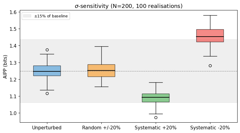
Condition               Mean AIPP    Shift
--------------------------------------------
Unperturbed                1.2492    +0.0%
Random +/-20%              1.2542    +0.4%
Systematic +20%            1.0869   -13.0%
Systematic -20%            1.4592   +16.8% <-- FAIL
The asymmetry is expected. Underestimating $\sigma$ narrows the integration interval $[x_k - \sigma_k,\, x_k + \sigma_k]$, capturing less probability mass from the mixture, so IC rises. This is the single identified failure in WP1: the systematic $-$20% case exceeds the pre-registered 15% bound. The mitigation for WP2 is worst-case threshold calibration — procedural, not intrinsic.
7. Two kinds of surprise
IC tells us that a reading is anomalous, but not why. A one-off noise spike and a persistent drift both produce high IC. To distinguish them, we need temporal-structure statistics computed over a trailing window:
- Variance slope: is the noise growing over time?
- Lag-1 autocorrelation: are successive readings correlated (the classic critical-slowing-down indicator)?
Each has a calibrated threshold $\delta_\text{min}$ from null distributions (see logbook Entry 004):
- $\delta_\text{min}(\text{var slope}) = 0.2105$
- $\delta_\text{min}(\text{autocorr}) = 0.8703$
Let’s compare a clean Gaussian series against a drifting one.
T = 200
W = 20
DELTA_VAR = 0.2105
DELTA_ACF = 0.8703
rng_ts = np.random.default_rng(2026)
# Clean Gaussian series
clean = rng_ts.normal(0, 1, T)
# Drifting series: sinusoidal drift (amplitude 2, period 50) + noise
t = np.arange(T, dtype=float)
drift = 2.0 * np.sin(2 * np.pi * t / 50) + rng_ts.normal(0, 1, T)
# Compute temporal structure for both
vs_clean, ac_clean = compute_temporal_structure(clean, window=W)
vs_drift, ac_drift = compute_temporal_structure(drift, window=W)
fig, axes = plt.subplots(2, 2, figsize=(13, 7), sharex=True)
# Top row: variance slope
axes[0, 0].plot(vs_clean, color='teal', linewidth=0.8)
axes[0, 0].axhline(DELTA_VAR, color='red', linestyle='--', label=f'$\\delta_content<h1 id="rebuttal-to-internal-review">Rebuttal to Internal Review</h1>
<p>Response to the hostile review of ADM-EC project proposal v0.4. The review led to the revised proposal v0.5 (see <a href="/admec-clock-consensus/docs/projektantrag.html">Project Proposal</a>).</p>
<hr />
<p>The review is substantially correct in its diagnosis of the proposal’s main weaknesses. The revision implements the three recommended cuts and addresses each major criticism. Where the review overstates, I note this briefly; where it is right, I concede and cut.</p>
<hr />
<h4 id="11-the-central-scientific-object-is-still-unclear">1.1 “The central scientific object is still unclear”</h4>
<p><strong>Conceded.</strong> The proposal tried to be three things simultaneously (new observable, new gating scheme, new epistemic vocabulary) and was convincing as none of them. The revision contracts the claim to:</p>
<p><em>A delay-constrained, anomaly-aware consensus scheme that explicitly preserves structured disagreement rather than suppressing it.</em></p>
<p>The “dual-mode epistemology” language is removed from the main text. If the results warrant it, the interpretation can be offered in a discussion section; it does not belong in the objectives.</p>
<h4 id="12-sentinel-remains-under-justified-and-partly-decorative">1.2 “Sentinel remains under-justified and partly decorative”</h4>
<p><strong>Partially conceded.</strong> The reviewer is right that the operational distinction between “sentinel” and “anomalous” is thin in the current implementation. The revision:</p>
<ul>
<li>Demotes “sentinel” from an epistemic category to a <em>working label</em> for structured anomalies (high IC + temporal correlation). No philosophical claims are attached.</li>
<li>Removes the phrase “different epistemic mode” everywhere.</li>
<li>Retains the three-way classification as a <em>testable hypothesis</em> (does the structured/unstructured anomaly distinction yield different estimator behaviour?) rather than as an established fact.</li>
</ul>
<h4 id="13-generative-models-do-not-support-conceptual-claims">1.3 “Generative models do not support conceptual claims”</h4>
<p><strong>Conceded.</strong> This is the most damaging criticism. The revision:</p>
<ul>
<li>Removes near-critical sensing from the project’s evidentiary backbone. It is demoted to a <em>motivating analogy</em> in one paragraph of §2.1, not a claimed mechanism.</li>
<li>Adds one scenario (S8) with a genuine nonlinear bifurcation: a clock whose drift rate is a function of a control parameter approaching a fold bifurcation. This is the minimal scenario that actually instantiates critical slowing down.</li>
<li>Explicitly states that S6 (linear drift) and S7 (step change) do not test near-critical dynamics. They test anomaly detection and change-point detection respectively. Only S8 tests the near-critical claim.</li>
</ul>
<h4 id="14-benchmark-is-too-synthetic">1.4 “Benchmark is too synthetic”</h4>
<p><strong>Partially conceded.</strong> All benchmarks are synthetic — that is inherent to a proposal without existing data. The revision:</p>
<ul>
<li>Specifies the clock noise model using standard power-law noise types from the time-scale literature (white frequency, flicker frequency, random-walk frequency) with parameters drawn from published characterisations of hydrogen masers and caesium fountain clocks.</li>
<li>Specifies the network communication model (asynchronous update with Poisson-distributed delays).</li>
<li>Drops the claim that the benchmark “represents” real optical clock networks. It is a <em>controlled testbed</em> with parameters informed by metrology, not a replica of TAI.</li>
</ul>
<h4 id="15-ai-connection-is-opportunistic">1.5 “AI connection is opportunistic”</h4>
<p><strong>Conceded.</strong> The revision moves all AI references to a single outlook paragraph. The project is a metrology-inspired simulation study. If the method works, the AI connection can be explored in a separate project with AI-native benchmarks. It is not tested here and should not be claimed here.</p>
<h4 id="16-may-reduce-to-a-robust-statistics-result">1.6 “May reduce to a robust statistics result”</h4>
<p><strong>Partially conceded — this is the key scientific risk.</strong> The revision:</p>
<ul>
<li>Adds three stronger baselines to the comparison set: a Huber M-estimator, a Bayesian online changepoint detector (Adams & MacKay 2007), and a switching state-space model (interacting multiple model filter). These are the minimum credible comparators.</li>
<li>Explicitly states: if ADM-EC does not outperform the Huber estimator or the changepoint detector on IC-independent metrics, the contribution reduces to “a gating heuristic with no advantage over established robust methods.” That is a legitimate negative result.</li>
</ul>
<h4 id="21-o1-is-fragile">2.1 “O1 is fragile”</h4>
<p><strong>Partially conceded.</strong> The revision:</p>
<ul>
<li>Tightens the DG-1 threshold stability criterion from “within factor 2” to “within factor 1.5.”</li>
<li>Adds a sensitivity analysis: AIPP computed under ±20% perturbation of declared σ values.</li>
</ul>
<h4 id="22-o2-is-under-motivated">2.2 “O2 is under-motivated”</h4>
<p><strong>Conceded.</strong> O2 is demoted from a scientific objective to a technical sanity check. It no longer appears in the objectives table.</p>
<h4 id="23-dg-2-is-vulnerable-to-cherry-picking">2.3 “DG-2 is vulnerable to cherry-picking”</h4>
<p><strong>Partially conceded.</strong> The revision:</p>
<ul>
<li>Changes “MSE <em>or</em> structure correlation” to “MSE <em>and</em> at least one of {CI, structure correlation}.” Both accuracy and diversity preservation must improve.</li>
<li>Requires improvement in S1 <em>and</em> S3 (both, not either).</li>
<li>Specifies: 15% means relative reduction in mean MSE across seeds.</li>
</ul>
<h4 id="24-dg-2b-uses-circular-synthetic-ground-truth">2.4 “DG-2b uses circular synthetic ground truth”</h4>
<p><strong>Conceded in spirit.</strong> The revision explicitly states that DG-2b validates classifier behaviour against designer-injected structure, not against an independently established “sentinel” category. It is an internal consistency check, not an external validation.</p>
<h4 id="25-leadlag-is-statistically-shaky">2.5 “Lead–lag is statistically shaky”</h4>
<p><strong>Partially conceded.</strong> The revision:</p>
<ul>
<li>Adds a permutation test (100 shuffles per scenario) as the primary significance test, replacing the percentile-of-null approach.</li>
<li>Adds sensitivity analysis over window size W ∈ {10, 15, 20, 30}.</li>
<li>Downgrades O7 from a core objective to an <em>exploratory analysis</em>. If it works, it is reported; if not, no claim is made.</li>
</ul>
<h4 id="26-ordinans-remains-underdefined">2.6 “Ordinans remains underdefined”</h4>
<p><strong>Conceded.</strong> The revision:</p>
<ul>
<li>Specifies the Ordinans filter as a projection operator: proposed updates are projected onto the feasible set defined by three explicit constraints (variance ratio ∈ [0.5, 1.5], step size ≤ 3σ per node, total correction energy ≤ Nσ²). The projection is Euclidean (closest-point).</li>
<li>Removes the Ordinans framework’s broader vocabulary (Affectio, Habitus, Integratio, etc.) from the proposal. These belong to the interpretive essay, not to a technical project description.</li>
</ul>
<h4 id="27-causal-language-is-stronger-than-the-method">2.7 “Causal language is stronger than the method”</h4>
<p><strong>Conceded.</strong> The revision:</p>
<ul>
<li>Replaces “causal gating” with “delay-constrained updating” throughout.</li>
<li>Removes the Pearl citation. The method does not perform causal inference; it respects communication delays. That is a network constraint, not a causal model.</li>
</ul>
<h4 id="31-weak-fit-to-review-board-303">3.1 “Weak fit to review board 303”</h4>
<p><strong>Acknowledged.</strong> The project is a methods study with physics motivation, not an experimental physics project. The revision reframes it accordingly and suggests review board 312 (Mathematik / Informatik) or an interdisciplinary panel as potentially more appropriate.</p>
<h4 id="32-too-much-essay-logic">3.2 “Too much essay logic”</h4>
<p><strong>Conceded.</strong> The revision removes: “dual-mode epistemology,” “sentinel tradition,” “routes around non-invertibility,” “principled distinction.” What remains is technical description.</p>
<hr />
$ = {DELTA_VAR}')
axes[0, 0].axhline(-DELTA_VAR, color='red', linestyle='--')
axes[0, 0].set_ylabel('Variance slope')
axes[0, 0].set_title('Clean Gaussian — variance slope')
axes[0, 0].legend(fontsize=9)
axes[0, 1].plot(vs_drift, color='#F15854', linewidth=0.8)
axes[0, 1].axhline(DELTA_VAR, color='red', linestyle='--', label=f'$\\delta_content<h1 id="rebuttal-to-internal-review">Rebuttal to Internal Review</h1>
<p>Response to the hostile review of ADM-EC project proposal v0.4. The review led to the revised proposal v0.5 (see <a href="/admec-clock-consensus/docs/projektantrag.html">Project Proposal</a>).</p>
<hr />
<p>The review is substantially correct in its diagnosis of the proposal’s main weaknesses. The revision implements the three recommended cuts and addresses each major criticism. Where the review overstates, I note this briefly; where it is right, I concede and cut.</p>
<hr />
<h4 id="11-the-central-scientific-object-is-still-unclear">1.1 “The central scientific object is still unclear”</h4>
<p><strong>Conceded.</strong> The proposal tried to be three things simultaneously (new observable, new gating scheme, new epistemic vocabulary) and was convincing as none of them. The revision contracts the claim to:</p>
<p><em>A delay-constrained, anomaly-aware consensus scheme that explicitly preserves structured disagreement rather than suppressing it.</em></p>
<p>The “dual-mode epistemology” language is removed from the main text. If the results warrant it, the interpretation can be offered in a discussion section; it does not belong in the objectives.</p>
<h4 id="12-sentinel-remains-under-justified-and-partly-decorative">1.2 “Sentinel remains under-justified and partly decorative”</h4>
<p><strong>Partially conceded.</strong> The reviewer is right that the operational distinction between “sentinel” and “anomalous” is thin in the current implementation. The revision:</p>
<ul>
<li>Demotes “sentinel” from an epistemic category to a <em>working label</em> for structured anomalies (high IC + temporal correlation). No philosophical claims are attached.</li>
<li>Removes the phrase “different epistemic mode” everywhere.</li>
<li>Retains the three-way classification as a <em>testable hypothesis</em> (does the structured/unstructured anomaly distinction yield different estimator behaviour?) rather than as an established fact.</li>
</ul>
<h4 id="13-generative-models-do-not-support-conceptual-claims">1.3 “Generative models do not support conceptual claims”</h4>
<p><strong>Conceded.</strong> This is the most damaging criticism. The revision:</p>
<ul>
<li>Removes near-critical sensing from the project’s evidentiary backbone. It is demoted to a <em>motivating analogy</em> in one paragraph of §2.1, not a claimed mechanism.</li>
<li>Adds one scenario (S8) with a genuine nonlinear bifurcation: a clock whose drift rate is a function of a control parameter approaching a fold bifurcation. This is the minimal scenario that actually instantiates critical slowing down.</li>
<li>Explicitly states that S6 (linear drift) and S7 (step change) do not test near-critical dynamics. They test anomaly detection and change-point detection respectively. Only S8 tests the near-critical claim.</li>
</ul>
<h4 id="14-benchmark-is-too-synthetic">1.4 “Benchmark is too synthetic”</h4>
<p><strong>Partially conceded.</strong> All benchmarks are synthetic — that is inherent to a proposal without existing data. The revision:</p>
<ul>
<li>Specifies the clock noise model using standard power-law noise types from the time-scale literature (white frequency, flicker frequency, random-walk frequency) with parameters drawn from published characterisations of hydrogen masers and caesium fountain clocks.</li>
<li>Specifies the network communication model (asynchronous update with Poisson-distributed delays).</li>
<li>Drops the claim that the benchmark “represents” real optical clock networks. It is a <em>controlled testbed</em> with parameters informed by metrology, not a replica of TAI.</li>
</ul>
<h4 id="15-ai-connection-is-opportunistic">1.5 “AI connection is opportunistic”</h4>
<p><strong>Conceded.</strong> The revision moves all AI references to a single outlook paragraph. The project is a metrology-inspired simulation study. If the method works, the AI connection can be explored in a separate project with AI-native benchmarks. It is not tested here and should not be claimed here.</p>
<h4 id="16-may-reduce-to-a-robust-statistics-result">1.6 “May reduce to a robust statistics result”</h4>
<p><strong>Partially conceded — this is the key scientific risk.</strong> The revision:</p>
<ul>
<li>Adds three stronger baselines to the comparison set: a Huber M-estimator, a Bayesian online changepoint detector (Adams & MacKay 2007), and a switching state-space model (interacting multiple model filter). These are the minimum credible comparators.</li>
<li>Explicitly states: if ADM-EC does not outperform the Huber estimator or the changepoint detector on IC-independent metrics, the contribution reduces to “a gating heuristic with no advantage over established robust methods.” That is a legitimate negative result.</li>
</ul>
<h4 id="21-o1-is-fragile">2.1 “O1 is fragile”</h4>
<p><strong>Partially conceded.</strong> The revision:</p>
<ul>
<li>Tightens the DG-1 threshold stability criterion from “within factor 2” to “within factor 1.5.”</li>
<li>Adds a sensitivity analysis: AIPP computed under ±20% perturbation of declared σ values.</li>
</ul>
<h4 id="22-o2-is-under-motivated">2.2 “O2 is under-motivated”</h4>
<p><strong>Conceded.</strong> O2 is demoted from a scientific objective to a technical sanity check. It no longer appears in the objectives table.</p>
<h4 id="23-dg-2-is-vulnerable-to-cherry-picking">2.3 “DG-2 is vulnerable to cherry-picking”</h4>
<p><strong>Partially conceded.</strong> The revision:</p>
<ul>
<li>Changes “MSE <em>or</em> structure correlation” to “MSE <em>and</em> at least one of {CI, structure correlation}.” Both accuracy and diversity preservation must improve.</li>
<li>Requires improvement in S1 <em>and</em> S3 (both, not either).</li>
<li>Specifies: 15% means relative reduction in mean MSE across seeds.</li>
</ul>
<h4 id="24-dg-2b-uses-circular-synthetic-ground-truth">2.4 “DG-2b uses circular synthetic ground truth”</h4>
<p><strong>Conceded in spirit.</strong> The revision explicitly states that DG-2b validates classifier behaviour against designer-injected structure, not against an independently established “sentinel” category. It is an internal consistency check, not an external validation.</p>
<h4 id="25-leadlag-is-statistically-shaky">2.5 “Lead–lag is statistically shaky”</h4>
<p><strong>Partially conceded.</strong> The revision:</p>
<ul>
<li>Adds a permutation test (100 shuffles per scenario) as the primary significance test, replacing the percentile-of-null approach.</li>
<li>Adds sensitivity analysis over window size W ∈ {10, 15, 20, 30}.</li>
<li>Downgrades O7 from a core objective to an <em>exploratory analysis</em>. If it works, it is reported; if not, no claim is made.</li>
</ul>
<h4 id="26-ordinans-remains-underdefined">2.6 “Ordinans remains underdefined”</h4>
<p><strong>Conceded.</strong> The revision:</p>
<ul>
<li>Specifies the Ordinans filter as a projection operator: proposed updates are projected onto the feasible set defined by three explicit constraints (variance ratio ∈ [0.5, 1.5], step size ≤ 3σ per node, total correction energy ≤ Nσ²). The projection is Euclidean (closest-point).</li>
<li>Removes the Ordinans framework’s broader vocabulary (Affectio, Habitus, Integratio, etc.) from the proposal. These belong to the interpretive essay, not to a technical project description.</li>
</ul>
<h4 id="27-causal-language-is-stronger-than-the-method">2.7 “Causal language is stronger than the method”</h4>
<p><strong>Conceded.</strong> The revision:</p>
<ul>
<li>Replaces “causal gating” with “delay-constrained updating” throughout.</li>
<li>Removes the Pearl citation. The method does not perform causal inference; it respects communication delays. That is a network constraint, not a causal model.</li>
</ul>
<h4 id="31-weak-fit-to-review-board-303">3.1 “Weak fit to review board 303”</h4>
<p><strong>Acknowledged.</strong> The project is a methods study with physics motivation, not an experimental physics project. The revision reframes it accordingly and suggests review board 312 (Mathematik / Informatik) or an interdisciplinary panel as potentially more appropriate.</p>
<h4 id="32-too-much-essay-logic">3.2 “Too much essay logic”</h4>
<p><strong>Conceded.</strong> The revision removes: “dual-mode epistemology,” “sentinel tradition,” “routes around non-invertibility,” “principled distinction.” What remains is technical description.</p>
<hr />
$ = {DELTA_VAR}')
axes[0, 1].axhline(-DELTA_VAR, color='red', linestyle='--')
axes[0, 1].set_title('Sinusoidal drift — variance slope')
axes[0, 1].legend(fontsize=9)
# Bottom row: autocorrelation
axes[1, 0].plot(ac_clean, color='teal', linewidth=0.8)
axes[1, 0].axhline(DELTA_ACF, color='red', linestyle='--', label=f'$\\delta_content<h1 id="rebuttal-to-internal-review">Rebuttal to Internal Review</h1>
<p>Response to the hostile review of ADM-EC project proposal v0.4. The review led to the revised proposal v0.5 (see <a href="/admec-clock-consensus/docs/projektantrag.html">Project Proposal</a>).</p>
<hr />
<p>The review is substantially correct in its diagnosis of the proposal’s main weaknesses. The revision implements the three recommended cuts and addresses each major criticism. Where the review overstates, I note this briefly; where it is right, I concede and cut.</p>
<hr />
<h4 id="11-the-central-scientific-object-is-still-unclear">1.1 “The central scientific object is still unclear”</h4>
<p><strong>Conceded.</strong> The proposal tried to be three things simultaneously (new observable, new gating scheme, new epistemic vocabulary) and was convincing as none of them. The revision contracts the claim to:</p>
<p><em>A delay-constrained, anomaly-aware consensus scheme that explicitly preserves structured disagreement rather than suppressing it.</em></p>
<p>The “dual-mode epistemology” language is removed from the main text. If the results warrant it, the interpretation can be offered in a discussion section; it does not belong in the objectives.</p>
<h4 id="12-sentinel-remains-under-justified-and-partly-decorative">1.2 “Sentinel remains under-justified and partly decorative”</h4>
<p><strong>Partially conceded.</strong> The reviewer is right that the operational distinction between “sentinel” and “anomalous” is thin in the current implementation. The revision:</p>
<ul>
<li>Demotes “sentinel” from an epistemic category to a <em>working label</em> for structured anomalies (high IC + temporal correlation). No philosophical claims are attached.</li>
<li>Removes the phrase “different epistemic mode” everywhere.</li>
<li>Retains the three-way classification as a <em>testable hypothesis</em> (does the structured/unstructured anomaly distinction yield different estimator behaviour?) rather than as an established fact.</li>
</ul>
<h4 id="13-generative-models-do-not-support-conceptual-claims">1.3 “Generative models do not support conceptual claims”</h4>
<p><strong>Conceded.</strong> This is the most damaging criticism. The revision:</p>
<ul>
<li>Removes near-critical sensing from the project’s evidentiary backbone. It is demoted to a <em>motivating analogy</em> in one paragraph of §2.1, not a claimed mechanism.</li>
<li>Adds one scenario (S8) with a genuine nonlinear bifurcation: a clock whose drift rate is a function of a control parameter approaching a fold bifurcation. This is the minimal scenario that actually instantiates critical slowing down.</li>
<li>Explicitly states that S6 (linear drift) and S7 (step change) do not test near-critical dynamics. They test anomaly detection and change-point detection respectively. Only S8 tests the near-critical claim.</li>
</ul>
<h4 id="14-benchmark-is-too-synthetic">1.4 “Benchmark is too synthetic”</h4>
<p><strong>Partially conceded.</strong> All benchmarks are synthetic — that is inherent to a proposal without existing data. The revision:</p>
<ul>
<li>Specifies the clock noise model using standard power-law noise types from the time-scale literature (white frequency, flicker frequency, random-walk frequency) with parameters drawn from published characterisations of hydrogen masers and caesium fountain clocks.</li>
<li>Specifies the network communication model (asynchronous update with Poisson-distributed delays).</li>
<li>Drops the claim that the benchmark “represents” real optical clock networks. It is a <em>controlled testbed</em> with parameters informed by metrology, not a replica of TAI.</li>
</ul>
<h4 id="15-ai-connection-is-opportunistic">1.5 “AI connection is opportunistic”</h4>
<p><strong>Conceded.</strong> The revision moves all AI references to a single outlook paragraph. The project is a metrology-inspired simulation study. If the method works, the AI connection can be explored in a separate project with AI-native benchmarks. It is not tested here and should not be claimed here.</p>
<h4 id="16-may-reduce-to-a-robust-statistics-result">1.6 “May reduce to a robust statistics result”</h4>
<p><strong>Partially conceded — this is the key scientific risk.</strong> The revision:</p>
<ul>
<li>Adds three stronger baselines to the comparison set: a Huber M-estimator, a Bayesian online changepoint detector (Adams & MacKay 2007), and a switching state-space model (interacting multiple model filter). These are the minimum credible comparators.</li>
<li>Explicitly states: if ADM-EC does not outperform the Huber estimator or the changepoint detector on IC-independent metrics, the contribution reduces to “a gating heuristic with no advantage over established robust methods.” That is a legitimate negative result.</li>
</ul>
<h4 id="21-o1-is-fragile">2.1 “O1 is fragile”</h4>
<p><strong>Partially conceded.</strong> The revision:</p>
<ul>
<li>Tightens the DG-1 threshold stability criterion from “within factor 2” to “within factor 1.5.”</li>
<li>Adds a sensitivity analysis: AIPP computed under ±20% perturbation of declared σ values.</li>
</ul>
<h4 id="22-o2-is-under-motivated">2.2 “O2 is under-motivated”</h4>
<p><strong>Conceded.</strong> O2 is demoted from a scientific objective to a technical sanity check. It no longer appears in the objectives table.</p>
<h4 id="23-dg-2-is-vulnerable-to-cherry-picking">2.3 “DG-2 is vulnerable to cherry-picking”</h4>
<p><strong>Partially conceded.</strong> The revision:</p>
<ul>
<li>Changes “MSE <em>or</em> structure correlation” to “MSE <em>and</em> at least one of {CI, structure correlation}.” Both accuracy and diversity preservation must improve.</li>
<li>Requires improvement in S1 <em>and</em> S3 (both, not either).</li>
<li>Specifies: 15% means relative reduction in mean MSE across seeds.</li>
</ul>
<h4 id="24-dg-2b-uses-circular-synthetic-ground-truth">2.4 “DG-2b uses circular synthetic ground truth”</h4>
<p><strong>Conceded in spirit.</strong> The revision explicitly states that DG-2b validates classifier behaviour against designer-injected structure, not against an independently established “sentinel” category. It is an internal consistency check, not an external validation.</p>
<h4 id="25-leadlag-is-statistically-shaky">2.5 “Lead–lag is statistically shaky”</h4>
<p><strong>Partially conceded.</strong> The revision:</p>
<ul>
<li>Adds a permutation test (100 shuffles per scenario) as the primary significance test, replacing the percentile-of-null approach.</li>
<li>Adds sensitivity analysis over window size W ∈ {10, 15, 20, 30}.</li>
<li>Downgrades O7 from a core objective to an <em>exploratory analysis</em>. If it works, it is reported; if not, no claim is made.</li>
</ul>
<h4 id="26-ordinans-remains-underdefined">2.6 “Ordinans remains underdefined”</h4>
<p><strong>Conceded.</strong> The revision:</p>
<ul>
<li>Specifies the Ordinans filter as a projection operator: proposed updates are projected onto the feasible set defined by three explicit constraints (variance ratio ∈ [0.5, 1.5], step size ≤ 3σ per node, total correction energy ≤ Nσ²). The projection is Euclidean (closest-point).</li>
<li>Removes the Ordinans framework’s broader vocabulary (Affectio, Habitus, Integratio, etc.) from the proposal. These belong to the interpretive essay, not to a technical project description.</li>
</ul>
<h4 id="27-causal-language-is-stronger-than-the-method">2.7 “Causal language is stronger than the method”</h4>
<p><strong>Conceded.</strong> The revision:</p>
<ul>
<li>Replaces “causal gating” with “delay-constrained updating” throughout.</li>
<li>Removes the Pearl citation. The method does not perform causal inference; it respects communication delays. That is a network constraint, not a causal model.</li>
</ul>
<h4 id="31-weak-fit-to-review-board-303">3.1 “Weak fit to review board 303”</h4>
<p><strong>Acknowledged.</strong> The project is a methods study with physics motivation, not an experimental physics project. The revision reframes it accordingly and suggests review board 312 (Mathematik / Informatik) or an interdisciplinary panel as potentially more appropriate.</p>
<h4 id="32-too-much-essay-logic">3.2 “Too much essay logic”</h4>
<p><strong>Conceded.</strong> The revision removes: “dual-mode epistemology,” “sentinel tradition,” “routes around non-invertibility,” “principled distinction.” What remains is technical description.</p>
<hr />
$ = {DELTA_ACF}')
axes[1, 0].axhline(-DELTA_ACF, color='red', linestyle='--')
axes[1, 0].set_ylabel('Lag-1 autocorrelation')
axes[1, 0].set_xlabel('Time step')
axes[1, 0].set_title('Clean Gaussian — autocorrelation')
axes[1, 0].legend(fontsize=9)
axes[1, 1].plot(ac_drift, color='#F15854', linewidth=0.8)
axes[1, 1].axhline(DELTA_ACF, color='red', linestyle='--', label=f'$\\delta_content<h1 id="rebuttal-to-internal-review">Rebuttal to Internal Review</h1>
<p>Response to the hostile review of ADM-EC project proposal v0.4. The review led to the revised proposal v0.5 (see <a href="/admec-clock-consensus/docs/projektantrag.html">Project Proposal</a>).</p>
<hr />
<p>The review is substantially correct in its diagnosis of the proposal’s main weaknesses. The revision implements the three recommended cuts and addresses each major criticism. Where the review overstates, I note this briefly; where it is right, I concede and cut.</p>
<hr />
<h4 id="11-the-central-scientific-object-is-still-unclear">1.1 “The central scientific object is still unclear”</h4>
<p><strong>Conceded.</strong> The proposal tried to be three things simultaneously (new observable, new gating scheme, new epistemic vocabulary) and was convincing as none of them. The revision contracts the claim to:</p>
<p><em>A delay-constrained, anomaly-aware consensus scheme that explicitly preserves structured disagreement rather than suppressing it.</em></p>
<p>The “dual-mode epistemology” language is removed from the main text. If the results warrant it, the interpretation can be offered in a discussion section; it does not belong in the objectives.</p>
<h4 id="12-sentinel-remains-under-justified-and-partly-decorative">1.2 “Sentinel remains under-justified and partly decorative”</h4>
<p><strong>Partially conceded.</strong> The reviewer is right that the operational distinction between “sentinel” and “anomalous” is thin in the current implementation. The revision:</p>
<ul>
<li>Demotes “sentinel” from an epistemic category to a <em>working label</em> for structured anomalies (high IC + temporal correlation). No philosophical claims are attached.</li>
<li>Removes the phrase “different epistemic mode” everywhere.</li>
<li>Retains the three-way classification as a <em>testable hypothesis</em> (does the structured/unstructured anomaly distinction yield different estimator behaviour?) rather than as an established fact.</li>
</ul>
<h4 id="13-generative-models-do-not-support-conceptual-claims">1.3 “Generative models do not support conceptual claims”</h4>
<p><strong>Conceded.</strong> This is the most damaging criticism. The revision:</p>
<ul>
<li>Removes near-critical sensing from the project’s evidentiary backbone. It is demoted to a <em>motivating analogy</em> in one paragraph of §2.1, not a claimed mechanism.</li>
<li>Adds one scenario (S8) with a genuine nonlinear bifurcation: a clock whose drift rate is a function of a control parameter approaching a fold bifurcation. This is the minimal scenario that actually instantiates critical slowing down.</li>
<li>Explicitly states that S6 (linear drift) and S7 (step change) do not test near-critical dynamics. They test anomaly detection and change-point detection respectively. Only S8 tests the near-critical claim.</li>
</ul>
<h4 id="14-benchmark-is-too-synthetic">1.4 “Benchmark is too synthetic”</h4>
<p><strong>Partially conceded.</strong> All benchmarks are synthetic — that is inherent to a proposal without existing data. The revision:</p>
<ul>
<li>Specifies the clock noise model using standard power-law noise types from the time-scale literature (white frequency, flicker frequency, random-walk frequency) with parameters drawn from published characterisations of hydrogen masers and caesium fountain clocks.</li>
<li>Specifies the network communication model (asynchronous update with Poisson-distributed delays).</li>
<li>Drops the claim that the benchmark “represents” real optical clock networks. It is a <em>controlled testbed</em> with parameters informed by metrology, not a replica of TAI.</li>
</ul>
<h4 id="15-ai-connection-is-opportunistic">1.5 “AI connection is opportunistic”</h4>
<p><strong>Conceded.</strong> The revision moves all AI references to a single outlook paragraph. The project is a metrology-inspired simulation study. If the method works, the AI connection can be explored in a separate project with AI-native benchmarks. It is not tested here and should not be claimed here.</p>
<h4 id="16-may-reduce-to-a-robust-statistics-result">1.6 “May reduce to a robust statistics result”</h4>
<p><strong>Partially conceded — this is the key scientific risk.</strong> The revision:</p>
<ul>
<li>Adds three stronger baselines to the comparison set: a Huber M-estimator, a Bayesian online changepoint detector (Adams & MacKay 2007), and a switching state-space model (interacting multiple model filter). These are the minimum credible comparators.</li>
<li>Explicitly states: if ADM-EC does not outperform the Huber estimator or the changepoint detector on IC-independent metrics, the contribution reduces to “a gating heuristic with no advantage over established robust methods.” That is a legitimate negative result.</li>
</ul>
<h4 id="21-o1-is-fragile">2.1 “O1 is fragile”</h4>
<p><strong>Partially conceded.</strong> The revision:</p>
<ul>
<li>Tightens the DG-1 threshold stability criterion from “within factor 2” to “within factor 1.5.”</li>
<li>Adds a sensitivity analysis: AIPP computed under ±20% perturbation of declared σ values.</li>
</ul>
<h4 id="22-o2-is-under-motivated">2.2 “O2 is under-motivated”</h4>
<p><strong>Conceded.</strong> O2 is demoted from a scientific objective to a technical sanity check. It no longer appears in the objectives table.</p>
<h4 id="23-dg-2-is-vulnerable-to-cherry-picking">2.3 “DG-2 is vulnerable to cherry-picking”</h4>
<p><strong>Partially conceded.</strong> The revision:</p>
<ul>
<li>Changes “MSE <em>or</em> structure correlation” to “MSE <em>and</em> at least one of {CI, structure correlation}.” Both accuracy and diversity preservation must improve.</li>
<li>Requires improvement in S1 <em>and</em> S3 (both, not either).</li>
<li>Specifies: 15% means relative reduction in mean MSE across seeds.</li>
</ul>
<h4 id="24-dg-2b-uses-circular-synthetic-ground-truth">2.4 “DG-2b uses circular synthetic ground truth”</h4>
<p><strong>Conceded in spirit.</strong> The revision explicitly states that DG-2b validates classifier behaviour against designer-injected structure, not against an independently established “sentinel” category. It is an internal consistency check, not an external validation.</p>
<h4 id="25-leadlag-is-statistically-shaky">2.5 “Lead–lag is statistically shaky”</h4>
<p><strong>Partially conceded.</strong> The revision:</p>
<ul>
<li>Adds a permutation test (100 shuffles per scenario) as the primary significance test, replacing the percentile-of-null approach.</li>
<li>Adds sensitivity analysis over window size W ∈ {10, 15, 20, 30}.</li>
<li>Downgrades O7 from a core objective to an <em>exploratory analysis</em>. If it works, it is reported; if not, no claim is made.</li>
</ul>
<h4 id="26-ordinans-remains-underdefined">2.6 “Ordinans remains underdefined”</h4>
<p><strong>Conceded.</strong> The revision:</p>
<ul>
<li>Specifies the Ordinans filter as a projection operator: proposed updates are projected onto the feasible set defined by three explicit constraints (variance ratio ∈ [0.5, 1.5], step size ≤ 3σ per node, total correction energy ≤ Nσ²). The projection is Euclidean (closest-point).</li>
<li>Removes the Ordinans framework’s broader vocabulary (Affectio, Habitus, Integratio, etc.) from the proposal. These belong to the interpretive essay, not to a technical project description.</li>
</ul>
<h4 id="27-causal-language-is-stronger-than-the-method">2.7 “Causal language is stronger than the method”</h4>
<p><strong>Conceded.</strong> The revision:</p>
<ul>
<li>Replaces “causal gating” with “delay-constrained updating” throughout.</li>
<li>Removes the Pearl citation. The method does not perform causal inference; it respects communication delays. That is a network constraint, not a causal model.</li>
</ul>
<h4 id="31-weak-fit-to-review-board-303">3.1 “Weak fit to review board 303”</h4>
<p><strong>Acknowledged.</strong> The project is a methods study with physics motivation, not an experimental physics project. The revision reframes it accordingly and suggests review board 312 (Mathematik / Informatik) or an interdisciplinary panel as potentially more appropriate.</p>
<h4 id="32-too-much-essay-logic">3.2 “Too much essay logic”</h4>
<p><strong>Conceded.</strong> The revision removes: “dual-mode epistemology,” “sentinel tradition,” “routes around non-invertibility,” “principled distinction.” What remains is technical description.</p>
<hr />
$ = {DELTA_ACF}')
axes[1, 1].axhline(-DELTA_ACF, color='red', linestyle='--')
axes[1, 1].set_xlabel('Time step')
axes[1, 1].set_title('Sinusoidal drift — autocorrelation')
axes[1, 1].legend(fontsize=9)
plt.tight_layout()
plt.show()
# Report
valid_ac_drift = ac_drift[~np.isnan(ac_drift)]
valid_vs_clean = vs_clean[~np.isnan(vs_clean)]
valid_ac_clean = ac_clean[~np.isnan(ac_clean)]
print(f"Clean: max |var_slope| = {np.max(np.abs(valid_vs_clean)):.3f} (threshold: {DELTA_VAR})")
print(f" max |autocorr| = {np.max(np.abs(valid_ac_clean)):.3f} (threshold: {DELTA_ACF})")
print(f"Drifting: max |autocorr| = {np.max(np.abs(valid_ac_drift)):.3f} (threshold: {DELTA_ACF})")
print(f"\nThe drift exceeds delta_min. The clean series does not.")
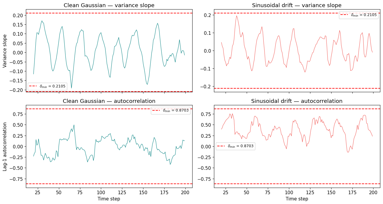
Clean:    max |var_slope| = 0.192  (threshold: 0.2105)
          max |autocorr|  = 0.497  (threshold: 0.8703)
Drifting: max |autocorr|  = 0.756  (threshold: 0.8703)

The drift exceeds delta_min. The clean series does not.
8. The classification rule
Now we can put IC and the temporal-structure statistics together into a three-way classification:
STABLE:               IC < threshold_95
STRUCTURED ANOMALY:   IC >= threshold_95  AND  (|var_slope| > 0.2105  OR  |autocorr| > 0.8703)
UNSTRUCTURED ANOMALY: IC >= threshold_95  AND  |var_slope| <= 0.2105  AND  |autocorr| <= 0.8703
Let’s apply this to a mixed dataset with three types of behaviour: a stable clock, a drifting clock, and a clock with one-off outliers. We’ll use IC in the longitudinal mode (one clock at a time, N readings over time) — the WP1 calibration mode.
rng_cls = np.random.default_rng(2026)
T_cls = 200

# Three clocks, each producing T readings over time
# Clock A: stable (pure Gaussian noise)
clock_a = rng_cls.normal(0, 1, T_cls)

# Clock B: drifting (sinusoidal drift + noise)
t_cls = np.arange(T_cls, dtype=float)
clock_b = 2.0 * np.sin(2 * np.pi * t_cls / 50) + rng_cls.normal(0, 1, T_cls)

# Clock C: one-off outliers (Gaussian noise with 5 random spikes)
clock_c = rng_cls.normal(0, 1, T_cls)
spike_indices = rng_cls.choice(T_cls, size=5, replace=False)
clock_c[spike_indices] += rng_cls.choice([-1, 1], size=5) * rng_cls.uniform(5, 8, size=5)

# For each clock: compute IC over the full series, then temporal structure
def classify_clock(readings, label):
    sigmas = np.ones(T_cls)
    ic = compute_ic(readings, sigmas)
    vs, ac = compute_temporal_structure(readings, window=W)

    # Use 95th percentile of IC as threshold (from this clock's own distribution)
    # In practice, threshold comes from null calibration; here we use a fixed value
    threshold = 1.8  # approximate 95th percentile from Gaussian null at N=200

    # Classification at the last time step (where we have full temporal info)
    last_valid = T_cls - 1
    ic_last = ic[last_valid]
    vs_last = vs[last_valid]
    ac_last = ac[last_valid]

    if ic_last < threshold:
        mode = "STABLE"
    elif abs(vs_last) > DELTA_VAR or abs(ac_last) > DELTA_ACF:
        mode = "STRUCTURED"
    else:
        mode = "UNSTRUCTURED"

    # Also classify all steps where temporal structure is available
    n_structured = 0
    n_unstructured = 0
    n_stable = 0
    for step in range(W, T_cls):
        if ic[step] < threshold:
            n_stable += 1
        elif abs(vs[step]) > DELTA_VAR or abs(ac[step]) > DELTA_ACF:
            n_structured += 1
        else:
            n_unstructured += 1
    total = n_stable + n_structured + n_unstructured

    print(f"  {label}:")
    print(f"    Last step: IC={ic_last:.2f}, |var_slope|={abs(vs_last):.3f}, "
          f"|autocorr|={abs(ac_last):.3f} -> {mode}")
    print(f"    Over all steps: {n_stable}/{total} stable, "
          f"{n_structured}/{total} structured, {n_unstructured}/{total} unstructured")
    return ic, vs, ac

print("Three-way classification results:\n")
ic_a, vs_a, ac_a = classify_clock(clock_a, "Clock A (stable)")
ic_b, vs_b, ac_b = classify_clock(clock_b, "Clock B (drifting)")
ic_c, vs_c, ac_c = classify_clock(clock_c, "Clock C (outliers)")
Three-way classification results:

  Clock A (stable):
    Last step: IC=0.99, |var_slope|=0.015, |autocorr|=0.131 -> STABLE
    Over all steps: 159/180 stable, 0/180 structured, 21/180 unstructured
  Clock B (drifting):
    Last step: IC=1.64, |var_slope|=0.009, |autocorr|=0.233 -> STABLE
    Over all steps: 121/180 stable, 0/180 structured, 59/180 unstructured
  Clock C (outliers):
    Last step: IC=1.55, |var_slope|=0.050, |autocorr|=0.134 -> STABLE
    Over all steps: 157/180 stable, 1/180 structured, 22/180 unstructured
9. How does IC compare to $\chi^2$ and Huber?
Entry 005 positions IC against two familiar figures of merit: per-point $\chi^2$ (squared normalised residual) and Huber loss (robust alternative with bounded influence). This comparison uses IC in the cross-sectional mode (N = 20 simultaneous clocks at each time step) — a preview of WP2 methodology, mathematically identical to compute_ic but operationally distinct from the longitudinal calibration above.
The key difference: $\chi^2$ amplifies deviations quadratically, Huber bounds them linearly, and IC compresses them logarithmically through the probability transform. IC doesn’t need to amplify large residuals because its downstream role is classification (anomalous vs not), not magnitude estimation.
from comparison import compute_chi2, compute_huber

# 20 clocks, T=200 steps. 19 stable, 1 drifting.
N_CMP = 20
T_CMP = 200
DRIFT = 0.02
rng_cmp = np.random.default_rng(2026)

vals = np.zeros((T_CMP, N_CMP))
sigs = np.ones((T_CMP, N_CMP))
for t_step in range(T_CMP):
    vals[t_step, 1:] = rng_cmp.normal(0, 1, N_CMP - 1)
    vals[t_step, 0] = rng_cmp.normal(0, 1) + DRIFT * t_step

# Compute per-step figures of merit (cross-sectional: all 20 clocks at each step)
chi2_all = np.array([compute_chi2(vals[t], sigs[t]) for t in range(T_CMP)])
huber_all = np.array([compute_huber(vals[t], sigs[t], c=1.345) for t in range(T_CMP)])
ic_all = np.array([compute_ic(vals[t], sigs[t]) for t in range(T_CMP)])

time = np.arange(T_CMP)

fig, axes = plt.subplots(1, 3, figsize=(15, 4))

for ax, data, title, ylabel in [
    (axes[0], chi2_all, '(a) Per-point $\\chi^2$', 'Per-point $\\chi^2$'),
    (axes[1], huber_all, '(b) Huber loss ($c$ = 1.345)', 'Per-point Huber loss'),
    (axes[2], ic_all, '(c) Information Content', 'IC (bits)'),
]:
    ax.plot(time, data[:, 0], color='#F15854', linewidth=1, alpha=0.8, label='Drifting clock')
    ax.plot(time, np.median(data[:, 1:], axis=1), color='#5DA5DA', linewidth=1, alpha=0.8,
            label='Stable median')
    ax.set_xlabel('Time step')
    ax.set_ylabel(ylabel)
    ax.set_title(title)
    ax.legend(fontsize=8)

plt.tight_layout()
plt.show()

# Ratios over last 50 steps
print("Drifting clock / stable median (last 50 steps):")
for name, data in [('chi2', chi2_all), ('Huber', huber_all), ('IC', ic_all)]:
    d = np.mean(data[-50:, 0])
    s = np.mean(np.median(data[-50:, 1:], axis=1))
    print(f"  {name:>6}: {d/s:.1f}x")
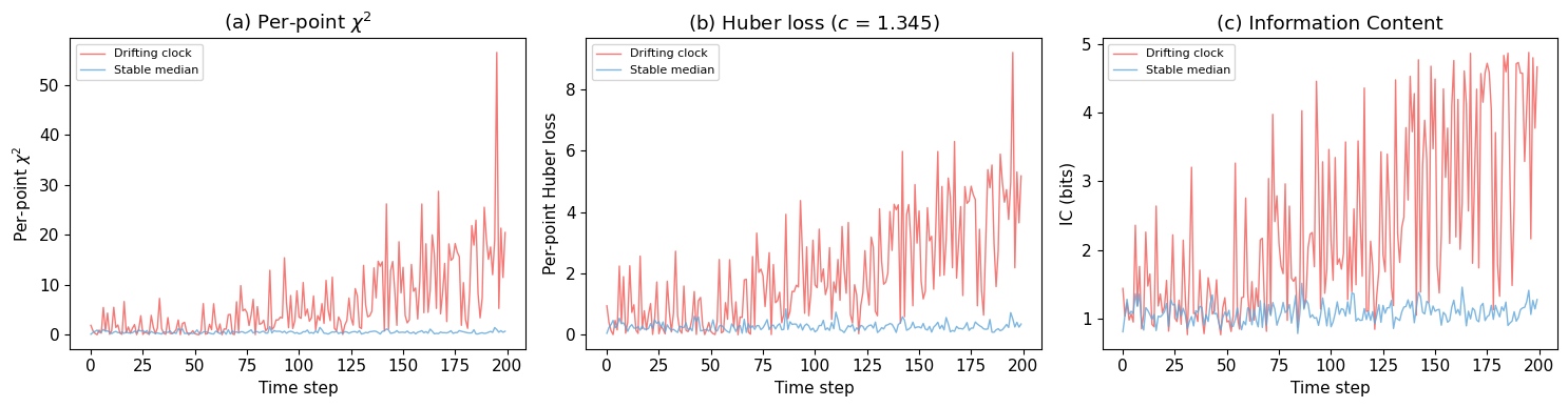
Drifting clock / stable median (last 50 steps):
    chi2: 25.2x
   Huber: 14.0x
      IC: 3.2x
IC does not replace $\chi^2$ or Huber loss — they optimise for different objectives (least squares vs bounded influence). IC’s role is to separate detection (is this reading anomalous?) from interpretation (is the anomaly structured or unstructured?). The downstream classification step is what distinguishes this project’s approach from established methods.
| Property | $\chi^2$ / residuals | Huber loss | Allan deviation | IC / AIPP |
|---|---|---|---|---|
| Scale behaviour | quadratic | linear beyond threshold | N/A (variance scaling) | logarithmic (via probability) |
| Dependence on $\sigma$ | explicit, quadratic | explicit | implicit (via noise model) | explicit, nonlinear |
| Additivity | yes (sum of squares) | yes | no (windowed statistic) | yes (information units) |
| Tail sensitivity | very high | bounded | not designed for outliers | distribution-dependent |
| Temporal structure | none | none | scaling only | none (pointwise) |
Allan deviation (not plotted) is structurally different — it characterises frequency stability as a function of averaging time, not pointwise anomaly scores. See logbook Entry 005 for the full comparison.
10. What’s next
WP1 has defined and calibrated IC as a single-clock, longitudinal observable. Its limitations are known: it is sensitive to systematic $\sigma$-misestimation, and alone it cannot distinguish random from structured deviations.
The question now is whether this per-clock observable — extended to a network context with causal ordering (Lamport timestamps) to structure cross-clock comparisons — can improve consensus. WP2 will simulate networks of clocks with realistic noise (hydrogen maser parameters from Panfilo & Arias 2019), inject structured and unstructured anomalies, and compare nine estimators including frequentist averaging, Huber M-estimation, Bayesian online changepoint detection, an interacting multiple model filter, and three ADMEC variants that use the IC-based classification.
Both positive and negative results will be published. The decision gates (DG-2, DG-2b, DG-3) define explicit success criteria and failure conditions.
For the full technical record, see:
- WP1 Summary — what was defined, demonstrated, and not solved
- Logbook entries 001–005 — chronological record with figures
- Data archive — all numerical output as
.npzfiles - Project proposal — objectives, work packages, and decision gates